2.4. CPLX Φ’s eigenvalues along the imaginary axisOnce the 3-dimensional histograms of fig. (3) are available, one can plot their 2-dimensional cross-sections along the imaginary axis. This is precisely the content of fig. (5). 
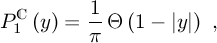
Figure 5: Histograms of the Φ’s eigenvalues along the imaginary axis This plot represents a bunch of 11 functions PC1(y), which in turn are cross-sections along the imaginary axis of the 3-dimensional histograms PC1(z) of fig. (3). The different colored lines represent the cases N=2 (red line), N=3,4,5,6,7,8,10,12 and N=14 (light-blue line). Finally, we plotted in dark-blue the Girko’s law,
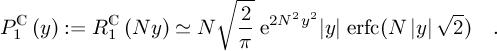
that we expect to hold for very large N, as already observed in fig. (3). We represent eq. (7) in the next fig. (6), for comparison with fig. (5). 
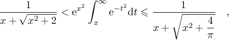
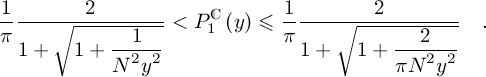
Figure 6: Theoretical distributions for the REAL Ginibre ensemble This plot represents a bunch of 11 distributions RC1(Ny) on the (rescaled) REAL Ginibre ensemble. The different colored lines represent the cases from N=2 (red line), N=3,4,5,6,7,8,10,12 and N=14 (light-blue line). From the formula (7.1.13) at page 298 of [AS72], that is together with eq. (7) and the definition of the complemetary error function erf(z), one can easily arrive at Such an inequality let a very few room to PC1(y), as one can see in the next fig. (7). 
Figure 7: Bound in the REAL Ginibre ensemble’s distributions The two bounds of eq. (9) are represented in dark-blue, together with PC1(y) (red line), for the case N=3. |