2.2. Distribution of the CPLX Φ’s Eigenvalues
Figure 2: Histograms of Φ’s Eigenvalues
This animated gif represents a sequence of 3
histograms of the complex eigenvalues of superoperators Φ,
distributed according to the measure induced by running the
Hans-Jürgen procedure. The sequence displays the cases N=2 (more
flat), N=3 and last N=4 (more peaked).
Fig. (2) displays a concentration
phenomenon. The higher N, the most concentrated the cloud of
eigenvalues toward the origin. Let now focus on the NC complex eigenvalues of Φ in the next fig. (3). 
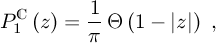
Figure 3: Histograms of Φ’s Eigenvalues This animated gif represents a sequence of 11 histograms of the complex eigenvalues of rescaled superoperators Φ, distributed according to the measure induced by running the Hans-Jürgen procedure. The sequence displays the cases N=2 (two symmetric bumps), N=3,4,5,6,7,8,10,12,14 and finally the so-called Girko’s law,
that we expect to hold for very large N (in the
plot we indicate such slide with N=infinity) |